6 Ways: Unique List of items from Multiple entries

Objective

You have some data where a particular field has many items occurring repeatedly and you need a list of unique items only like from (A,B,A,C,D,E,F,F,E,C,B,A,D) you need (A,B,C,D,E)

Prerequisites

There are six methods of doing it. Few may need Advance Excel / VBA basic knowledge.

Solution Concept

List can be created through Six different ways, no one is best but the one with whom the User is most comfortable. There are:

1.   Consolidate

2.   Advanced Filter

3.   Pivot Table

4.   Functions: COUNTIF, SMALL, INDIRECT

5.   Array

6.   Macro / VBA

Let’s do it

1.1.                Consolidate

1.1.1. This is what I am comfortable with and use.

1.1.2. I would add ‘1’ in front of each item in the list.

1.1.3. Then consolidate the two columns, based on Left Column

1.1.4. This will give me list of items along with number of their occurrence.

1.1.5. Occurrence column if not needed can be deleted and I am left with my unique entries

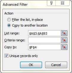
1.2.                Advanced Filter

1.2.1. While apply advanced filter choose (most commonly used):

            Copy to another location

            Unique records only

1.3.                Pivot Table

1.3.1. Select Column

1.3.2. Insert Pivot Table

1.3.3. Show data in rows

1.3.4. Copy / Value Paste Results

See Video

1.4.                Functions

1.4.1. This is dealt in separate post/lesson (Click here)

1.4.2. This solution is generally used when you need list to be created for a Macro

1.5.                Array Functions

1.5.1. This solution is available on many web sites, so I am unable to quote specific credit. This solution is definitely not developed or thought by me. You need to have concept of Arrays (Click here) to understand this.

1.5.2. The Equation:

“=INDEX($A$4:$A$93,MATCH(0,COUNTIF($C$3:C4,$A$4:$A$93),0))“

1.5.3. What I could understand:

  

   INDEX = Picks result from specific row and column in a Table

MATCH = Searches a specific text in a column and result in row number where result is found

COUNTIF = Counts number of occurrence

So first we count in “ABOVE” rows (Please check the reference $C$3:C4 – start is fixed, if you copy down, range will increase); this equation is entered in Row 5.

If the result is ‘0’ then Match will pick Row (As we are search in rows above so every entry will get at least one 0 occurrence)

INDEX picks results from Matched Row. I am not sure how Index changes the row to pick result from, when we drag and copy equation to multiple rows.

It is my understanding that when we make multiple rows part of an array; then inherent feature of array refers to next data item automatically.

1.5.4. Yes it is quite technical for me too, but programmers can grab it easily I believe.

1.6.                Macros / VBA

1.6.1. There are two macros in sample workbook, you check them with ‘a’ password

1.6.2. One Macro works with specific Range

1.6.3. The Other allows you to Pick the Range too

1.6.4. These macros need quite some explanation; so I have decided to do it in a separate post/lesson.

1.6.5. Meanwhile you can try to understand the code, which may be not very difficult for some.

1.6.6. Or you can use the code in your models by just changing the Range references.

Sample Workbook